Case Study 1: Collision Analysis: Analyzing the Blue Volkswagen and Red Volvo Collision
Part 1: Collision Analysis
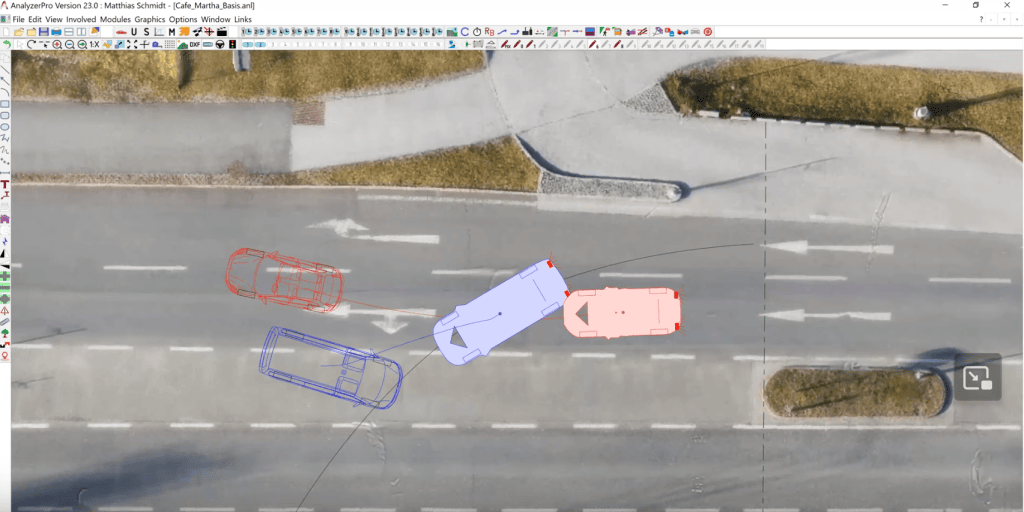
Introduction: In this case study, we examine a collision involving two vehicles: a blue Volkswagen and a red Volvo. The incident occurred when the blue car attempted to make a left turn across the road to park in front of a café. Unfortunately, the red car traveling in the same direction failed to notice the blue car’s turn early enough, resulting in a collision. We have obtained police photos that reveal damage to the front of the red car and the rear of the blue car. Our objective is to outline the steps involved in working on such a case and to determine the first course of action.


Step 1: Defining Participants. The initial step involves inputting vehicle data into AnalyzerPro. This can be done either manually or by utilizing the integrated database to select the two vehicles involved in the collision.
Step 2: Bringing in a Sketch. AnalyzerPro provides multiple options for creating a sketch of the collision. Users can directly draw using the available drawing tools or import photos by dragging and dropping them. Additionally, access to Google Maps is available. A modern and increasingly popular method is to use 3D photogrammetry or laser scans, which can be read into AnalyzerPro to generate both 2D images and 3D landscape representations.
Step 3: Establishing the Initial Conditions. In many cases, we have limited information about the collision. To compensate for this, we create an imaginary path that the blue car would have followed if the turn had gone uninterrupted. This path helps us estimate where the car would have been at the point of collision.
Our primary goal is to determine the collision speed of the two vehicles. Analyzer offers several methods for this, with momentum forward calculation being one of the most commonly used techniques. In this case, we are conducting an automatic collision analysis which relies on the same principles but speeds up the trial-and-error part drastically.
Automatic Collision Analysis: We open the module and see the five steps we have to take.
1. Specify Collision Positions: For the collision positions we are making an estimation. Note that the momentum forward calculation does require an overlap of the vehicles.
2. Specify End Positions: We have precise information about the final positions of the vehicles from the police photos.
3. Enter Parameters: This step involves providing input about what is known and what needs to be determined. We want the algorithm to calculates the tangent. We give typical ranges for the k-factor (impact elasticity) and coefficient of friction between the cars. Estimated speeds are input, with a range of 5 to 30 km/h for the blue car and 30 to 90 km/h for the red car. Brake pedal values are entered between 1 and 90% for both cars, and for the steering wheel, we consider a positive value for the blue car’s left turn.

In the bottom of the window, we can indicate that we do not have the exact positions of our collision. This is why we give the two cars relative shifts and rotations to their indicated positions: we specify a range or 5 cm and 5 degrees.
4. Calculate: The software performs a momentum forward collision analysis, requiring some time for computation. AnalyzerPro calculates automatically 10 different series of calculations that allow the user to see if there are different sets of input parameters that reach the same final position.
5. Display and Transfer: After obtaining results, necessary data can be selected and transferred to the collision analysis and kinematic windows.
Main Data Window: The main data window serves as an overview where all data is consolidated. It also enables the utilization of different techniques and approaches, allowing for comprehensive analysis and calculations, especially in kinematics.
Conclusion: By following these steps and utilizing AnalyzerPro, we can effectively analyze and reconstruct collision scenarios, assisting in determining collision speeds and contributing to a thorough understanding of the crash and post-crash behaviour.
Part 2: Pre-Collision Analysis
After our initial steps, we proceed with a Pre-Collision Analysis to gain a deeper understanding of why and how the accident occurred. To do this, we’ll use a specialized module for our blue car called the Turning Procedure Module, designed to simulate vehicles going around curves, allowing for acceleration during turns and more.
Blue Car Analysis:
We click on our Turning procedure module and open the window. Here we have to fill in our values:
Initial and Final Radius: The initial radius when the car was in its lane is 0, and the final radius when it was turning is approximately 15 meters, which we obtain by using the graphic tools.
Steering Time: We don’t have precise data, so we make an estimate of 1 to 2 seconds, considering different scenarios.
Maximum Yaw Angle: About 30 degrees.
Initial Velocity: Starting from 0.
Acceleration: Approximately 2 m/s².

Once these values are entered, we click “Calculate.” The software then computes missing values and displays the driving path of the blue car. An advantageous feature of Analyzer is its ability to adjust other values based on changes made, facilitating scenario exploration.

Clicking “Calculate” provides additional insights, including initial velocity, braking distance, braking time, total distance for reaction, build-up, and braking phases, as well as a missing braking distance of around 18 meters.
Red Car Analysis:
Moving on to the red car, we consider its reaction, build-up phase, and potential braking. To determine when the blue car becomes visible to the red car, we use the “Calculate Path Time” module. This module calculates the combination of reaction-, build-up and braking phase together when only a total distance or time is given. It requires five input values. In our case we fill in the following:
Reaction Period: Estimated between 1 to 0.8 seconds.
Build-up Time: Estimated at 0.2 seconds.
Final Velocity: Automatically obtained from the main data window, resulting from the previous collision analysis at 57.37 km/h.
Total Time: We check when the blue car is likely to be visible for the red one. This could be when the left front edge of the blue car is moving on to the lane of the red car. Using the time bar, it can be found out that this was approximately 1,3 seconds before impact. That means that the total time, aka the time available for reaction, build up and braking results in 1,3 seconds.
Deceleration: Estimated at 7 meters per square second, dependent on road conditions.
Visualizing in 3D: For a comprehensive view, we can visualize the entire scenario in 3D, allowing us to gain deeper insights into the spatial relationships and positions of the vehicles, just by clicking on the 3D button.
Conclusion: Through this Pre-Collision Analysis, we’ve examined the dynamics leading up to the accident, considering the blue car’s turning procedure and the red car’s reaction. This detailed analysis sheds light on the critical moments before the collision occurred.


Report Generation: Additionally, it’s important to note that Analyzer includes a report generation feature. By clicking on “File” and selecting “Create Report,” the software can generate a comprehensive report containing all input data, formulas, and calculations that led to the results. This report serves as a valuable resource for documentation and communication of findings in a clear and organized manner.
Case Study 2: Data Analysis - Digital Data in Collision Investigation
Introduction: In this case study, we encounter the growing significance of digital data in accident investigations. The case involves two key data sources: an Audi car equipped with Bosch CDR data and a truck fitted with digital tachograph data. The objective is to employ these data sources to comprehensively analyze the events leading up to a collision between the two vehicles.
Event Overview: According to witness testimonies, the chain of events unfolded as follows: The truck, aiming to enter the highway, swiftly shifted from the initial lane to the second lane and subsequently to the far-left lane (direction: left to right). Meanwhile, the Audi car was traveling at a high speed in the left lane. These actions culminated in a collision, as depicted in the accompanying image.


Analyzing the Truck’s Data:
Digital Tachograph Data: Across many European countries, regulations increasingly mandate the use of digital tachographs for vehicles weighing over 3.5 tonnes. These data files typically carry formats such as .ddd or .v1B, and Analyzer seamlessly reads these files, which contain speed data sampled at 1 Hertz (one speed value per second) or 4 Hertz.
(1) Data Import: The process begins by navigating to the “Modules” section, selecting “Import driving data,” and then choosing “DDD tachograph data.” The relevant DDD file is loaded, and we proceed to select the specific time period corresponding to the collision, which is the final recorded data point before the accident.
(2) Acceleration and Deceleration Analysis: Reviewing the data reveals instances of acceleration and subsequent deceleration. Given the substantial weight of the truck, the collision with the much lighter car has a limited impact on it. However, we assume that the truck reacted once the driver felt the impact. Consequently, we select a time range extending from just before the deceleration phase to a bit afterward, effectively isolating the critical pre-collision phase. This selected data is then transferred to the main data window.
(3) Synchronization: To pinpoint the collision point within the data, we hone in on phase 6, where the truck reached its highest speed. A second prior to this point, we assume the driver reacted, requiring that time to respond, subsequently engaging the brakes. To facilitate synchronization, we set position distance and position time to zero for phase 6. This means that everything before this point is represented as a positive value, and everything beyond is a negative value. This aids us in working from the most pivotal moment—namely, the collision.


(4) Validation: To confirm the feasibility of our interpretation from a physics standpoint, we refer to the Coordinates Window. This window provides detailed information about every point in the truck’s movement. We assess whether the lateral acceleration falls within acceptable limits, verifying the technical viability of the reconstructed scenario.
(5) Creating an Alternative Scenario: To explore an alternative scenario where the truck proceeds straight in its lane and changes lanes later, Analyzer allows for the creation of copies of vehicles. By copying vehicle data from the original truck to a new instance (e.g., vehicle number three), we can construct an alternative version of the truck’s path.

Analyzing the Red Car’s Data:
Moving on to the second vehicle, the red car, we encounter Bosch CDR data. Bosch CDR is a tool that reads vehicle systems, such as airbag modules, and stores pertinent data.
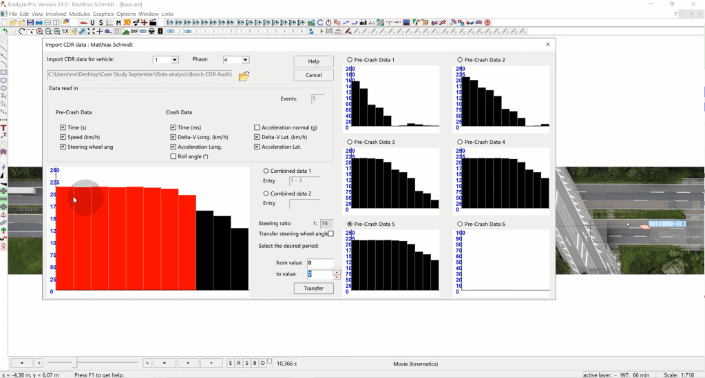
(1) Data Import: Within Analyzer, a dedicated module for Bosch CDR data is accessible via the “Modules” section, under “Import driving data.” We select the appropriate file format (e.g., CSV) and specify that this data pertains to vehicle 2.
(2) Data Selection: We assume that the accident happened at a certain data point that we select. The red part that you can see in the picture is before the collision and the black part is after the collision.
(3) Data Transfer: The chosen pre-crash data (in this case, event 5) is transferred, allowing us to recreate the pre-collision behavior of the red car.
(4) Synchronization: To synchronize the red car’s behavior with the collision event, we click on the flag symbol. Furthermore, adjustments are made to the driving line as needed.


Kinematic Data Analysis:
Examination of the kinematic data of the red car shows a phase of acceleration followed by deceleration. The beginning of the reaction occurs when the red car changes from acceleration to deceleration, about 1.5 seconds before point 0, which is the collision position. If we click on the clock symbol and enter 1.5, we see the scenery exactly 1.5 seconds before the collision. In our case, we can conclude that the red driver should have seen the blue truck earlier, which means that he could have reacted earlier.
Verifying Line of Sight: As part of the analysis, we consider the truck’s perspective. When changing lanes, it’s customary for drivers to check their mirrors. To account for this, we incorporate the truck’s left outer mirror using the lines of sight symbol in the menu. Settings are adjusted for the mirror, revealing a triangular field of vision on the truck. This visualization confirms that the red car should have been within the mirror’s lines of sight.
Conclusion: In conclusion, this comprehensive data analysis provides critical insights into the circumstances leading to the collision between the Audi car and the truck. Through meticulous examination of both digital tachograph and Bosch CDR data, we gain a clearer understanding of the events, driver reactions, and potential contributing factors surrounding this accident.